Carregando Bibliotecas
#>  default    student       balance           income
#>  No :9667   No :7056   Min.   :   0.0   Min.   :  772
#>  Yes: 333   Yes:2944   1st Qu.: 481.7   1st Qu.:21340
#>                        Median : 823.6   Median :34553
#>                        Mean   : 835.4   Mean   :33517
#>                        3rd Qu.:1166.3   3rd Qu.:43808
#>                        Max.   :2654.3   Max.   :73554
#> 'data.frame':    10000 obs. of  4 variables:
#>  $ default: Factor w/ 2 levels "No","Yes": 1 1 1 1 1 1 1 1 1 1 ...
#>  $ student: Factor w/ 2 levels "No","Yes": 1 2 1 1 1 2 1 2 1 1 ...
#>  $ balance: num  730 817 1074 529 786 ...
#>  $ income : num  44362 12106 31767 35704 38463 ...
#>   default student   balance    income
#> 1      No      No  729.5265 44361.625
#> 2      No     Yes  817.1804 12106.135
#> 3      No      No 1073.5492 31767.139
#> 4      No      No  529.2506 35704.494
#> 5      No      No  785.6559 38463.496
#> 6      No     Yes  919.5885  7491.559
Manipulando os dados
#>  default    student       balance           income
#>  No :9667   No :7056   Min.   :   0.0   Min.   :  772
#>  Yes: 333   Yes:2944   1st Qu.: 481.7   1st Qu.:21340
#>                        Median : 823.6   Median :34553
#>                        Mean   : 835.4   Mean   :33517
#>                        3rd Qu.:1166.3   3rd Qu.:43808
#>                        Max.   :2654.3   Max.   :73554
# renomeando colunas credito <- credito %>% rename ( inadimplente = default , estudante = student , balanco = balance ,
receita = income )
credito <- credito %>% mutate ( inadimplente = case_when ( inadimplente == "No" ~ "Nao" ,
inadimplente == "Yes" ~ "Sim"
) ) %>% mutate ( inadimplente = factor ( inadimplente ) )
credito <- credito %>% mutate ( estudante = case_when ( estudante == "No" ~ 0 ,
estudante == "Yes" ~ 1
) )
str ( credito )
#> tibble [10,000 × 4] (S3: tbl_df/tbl/data.frame)
#>  $ inadimplente: Factor w/ 2 levels "Nao","Sim": 1 1 1 1 1 1 1 1 1 1 ...
#>  $ estudante   : num [1:10000] 0 1 0 0 0 1 0 1 0 0 ...
#>  $ balanco     : num [1:10000] 730 817 1074 529 786 ...
#>  $ receita     : num [1:10000] 44362 12106 31767 35704 38463 ...
#>  inadimplente   estudante         balanco          receita
#>  Nao:9667     Min.   :0.0000   Min.   :   0.0   Min.   :  772
#>  Sim: 333     1st Qu.:0.0000   1st Qu.: 481.7   1st Qu.:21340
#>               Median :0.0000   Median : 823.6   Median :34553
#>               Mean   :0.2944   Mean   : 835.4   Mean   :33517
#>               3rd Qu.:1.0000   3rd Qu.:1166.3   3rd Qu.:43808
#>               Max.   :1.0000   Max.   :2654.3   Max.   :73554
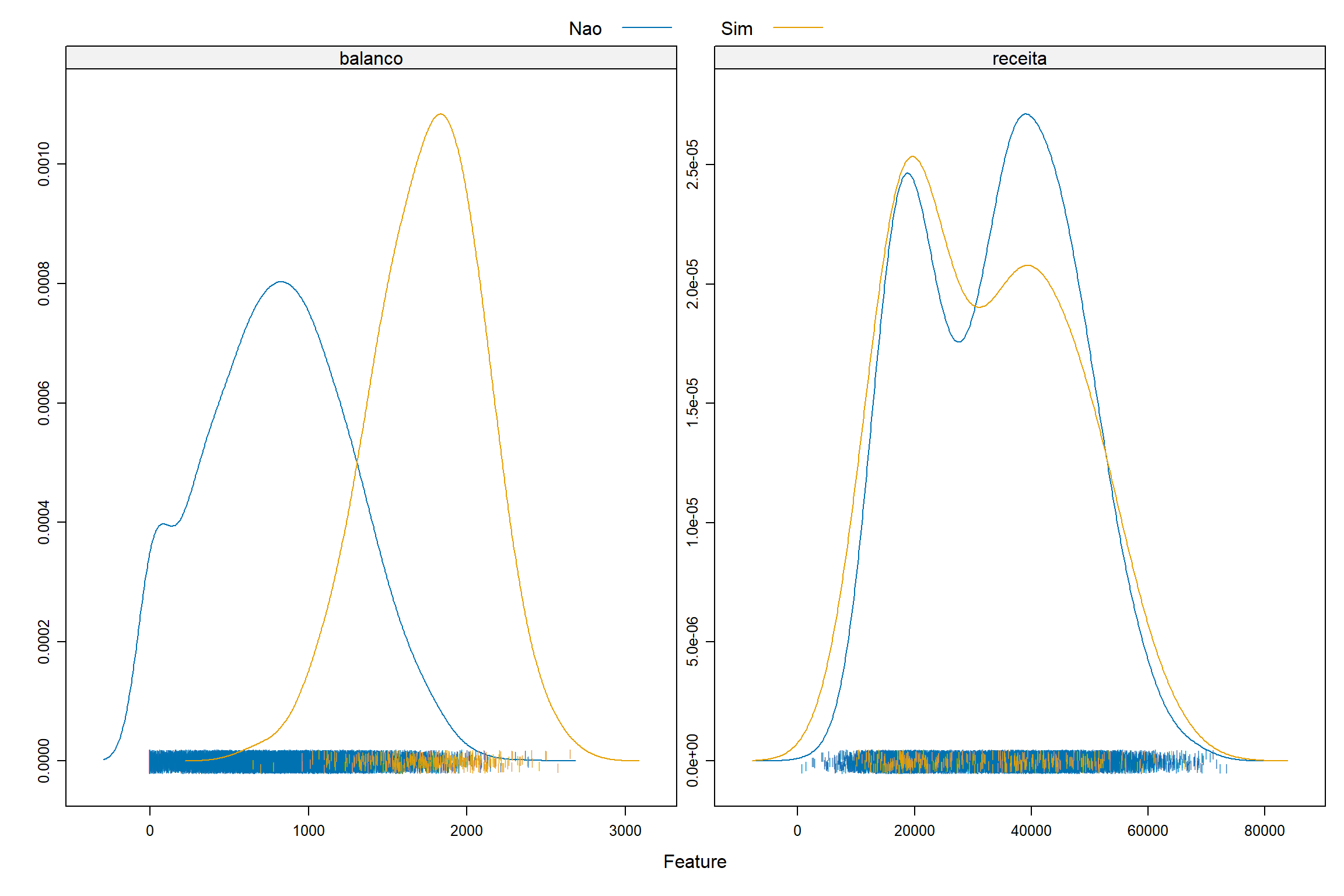
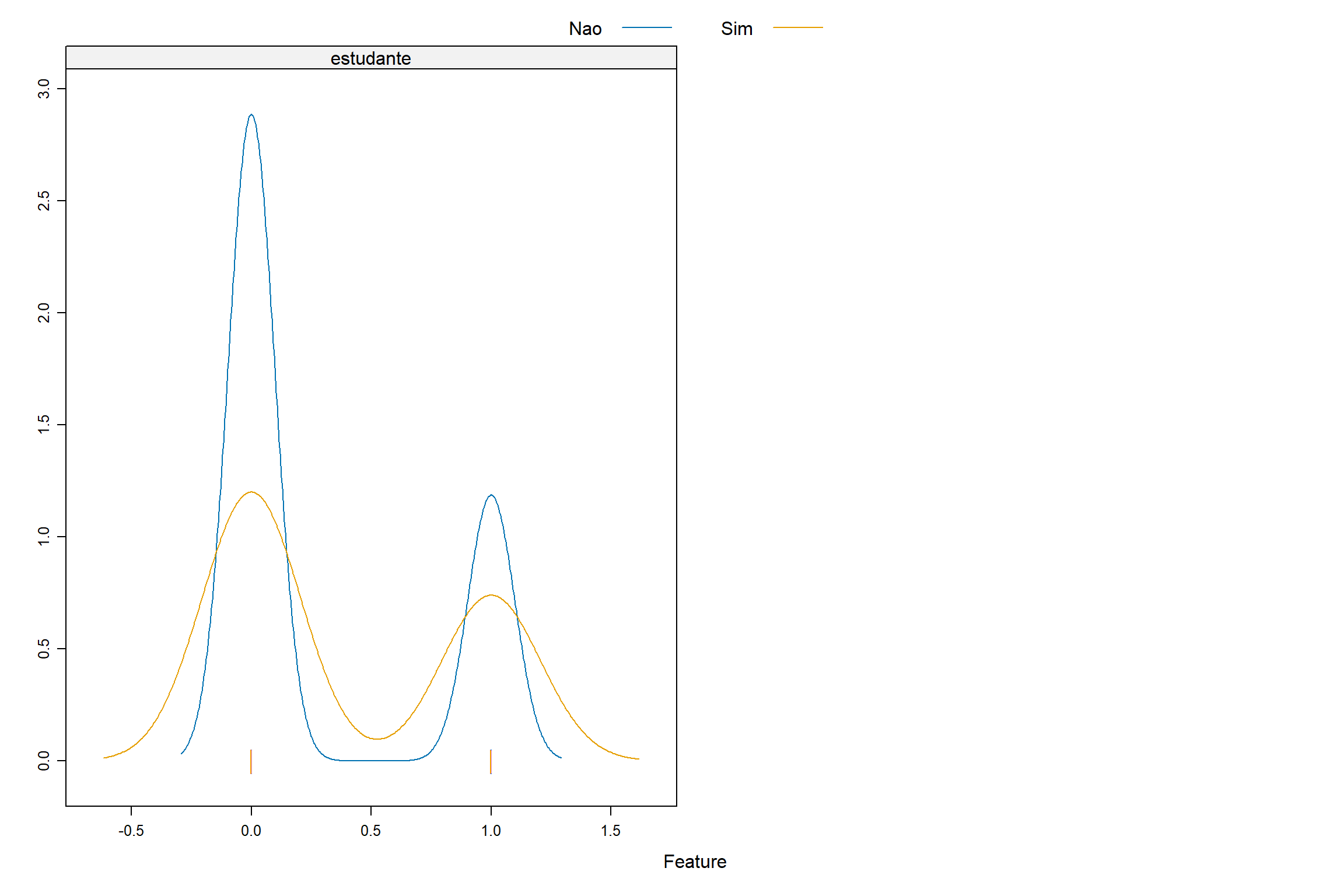
Graficos de Densidade
Vamos agora explorar os dados originais para termos algum visão do comportamento das variáveis explicativas e a variável dependente.
featurePlot ( x = credito [ , c ( "balanco" , "receita" , "estudante" ) ] , y = credito $ inadimplente ,
plot = "density" ,
scales = list ( x = list ( relation = "free" ) ,
y = list ( relation = "free" ) ) ,
adjust = 1.5 ,
pch = "|" ,
layout = c ( 2 , 1 ) ,
auto.key = list ( columns = 2 ) )
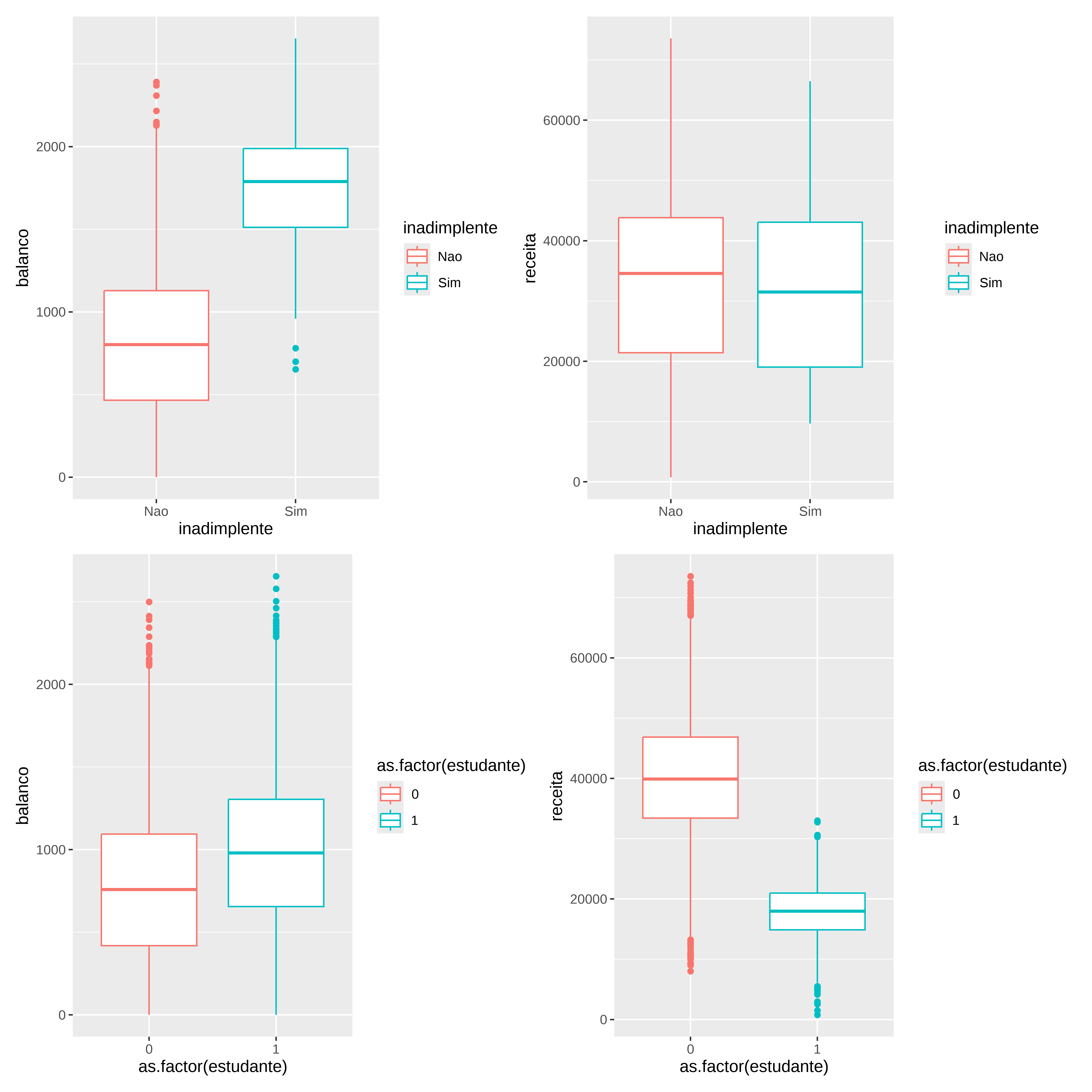
Avaliando o comportamento das variáveis em função do status (inadimplente / estudante)
p1 <- ggplot ( credito , aes ( x= inadimplente , y= balanco , color= inadimplente ) ) + geom_boxplot ( )
p2 <- ggplot ( credito , aes ( x= inadimplente , y= receita , color= inadimplente ) ) + geom_boxplot ( )
p3 <- ggplot ( credito , aes ( x= as.factor ( estudante ) , y= balanco , color= as.factor ( estudante ) ) ) + geom_boxplot ( )
p4 <- ggplot ( credito , aes ( x= as.factor ( estudante ) , y= receita , color= as.factor ( estudante ) ) ) + geom_boxplot ( )
( p1 + p2 ) / ( p3 + p4 )
Avaliando comportamento
#> # A tibble: 1 × 1
#>     prop
#>    <dbl>
#> 1 0.0333
#> # A tibble: 1 × 1
#>   valor
#>   <dbl>
#> 1 1748.
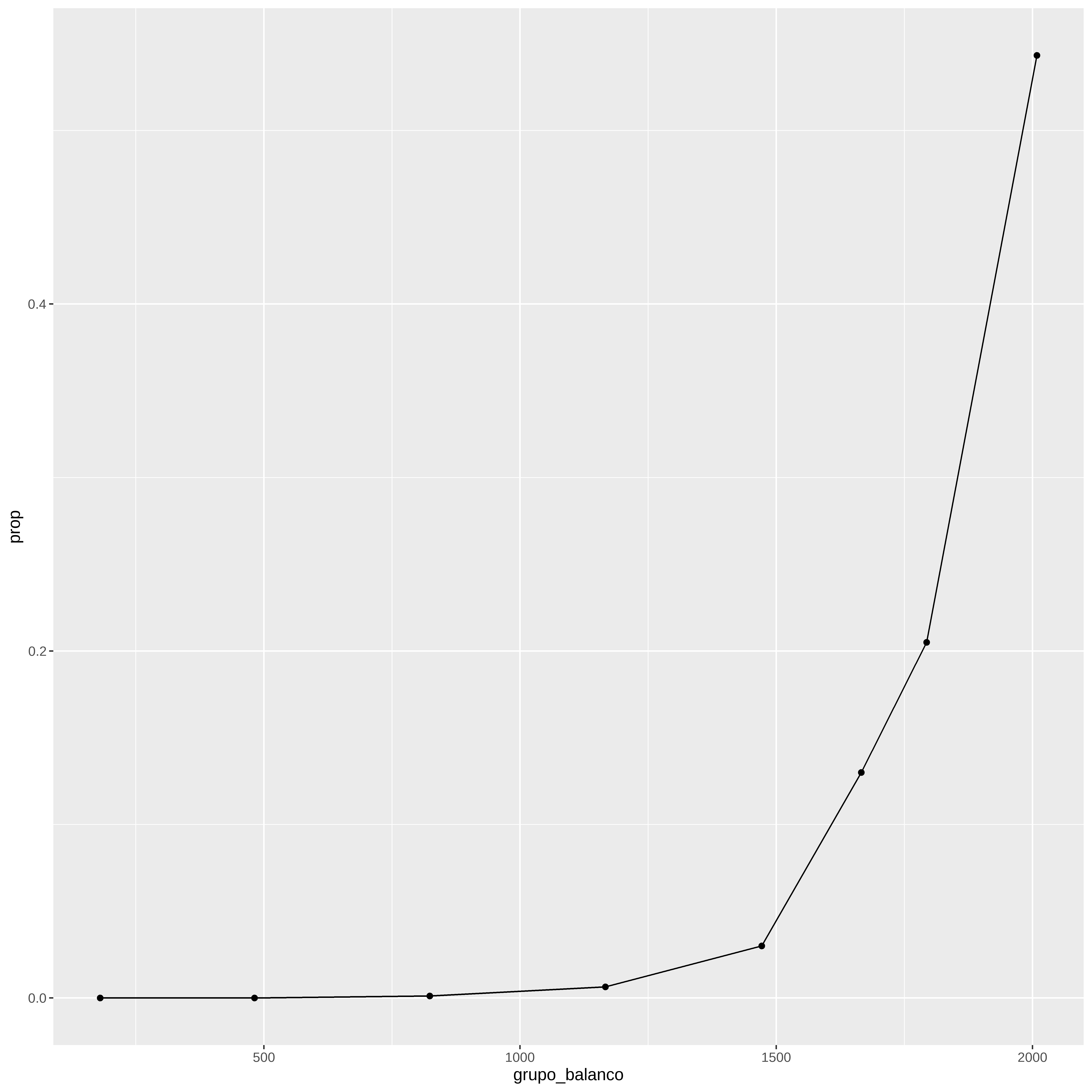
quantis <- quantile ( credito $ balanco , probs = c ( .1 ,.25 , .50 , .75 , .9 , .95 , 0.97 , 0.99 ) ) quantis
#>       10%       25%       50%       75%       90%       95%       97%       99%
#>  180.5753  481.7311  823.6370 1166.3084 1471.6253 1665.9626 1793.2910 2008.4709
credito %>% mutate ( grupo_balanco = case_when (
balanco <= quantis [ 1 ] ~ quantis [ 1 ] ,
balanco > quantis [ 1 ] & balanco <= quantis [ 2 ] ~ quantis [ 2 ] ,
balanco > quantis [ 2 ] & balanco <= quantis [ 3 ] ~ quantis [ 3 ] ,
balanco > quantis [ 3 ] & balanco <= quantis [ 4 ] ~ quantis [ 4 ] ,
balanco > quantis [ 4 ] & balanco <= quantis [ 5 ] ~ quantis [ 5 ] ,
balanco > quantis [ 5 ] & balanco <= quantis [ 6 ] ~ quantis [ 6 ] ,
balanco > quantis [ 6 ] & balanco <= quantis [ 7 ] ~ quantis [ 7 ] ,
balanco > quantis [ 7 ] ~ quantis [ 8 ] ) ) %>%
group_by ( grupo_balanco ) %>%
summarize ( prop = mean ( inadimplente == "Sim" ) ) %>%
ggplot ( aes ( grupo_balanco , prop ) ) +
geom_point ( ) +
geom_line ( )
Treino e Teste
set.seed ( 2025 ) y <- credito $ inadimplente credito_split <- createDataPartition ( y , times = 1 , p = 0.10 , list = FALSE ) conj_treino <- credito [ - credito_split ,] conj_teste <- credito [ credito_split ,]
summary ( conj_treino )
#>  inadimplente   estudante         balanco          receita
#>  Nao:8700     Min.   :0.0000   Min.   :   0.0   Min.   :  772
#>  Sim: 299     1st Qu.:0.0000   1st Qu.: 483.6   1st Qu.:21343
#>               Median :0.0000   Median : 821.3   Median :34576
#>               Mean   :0.2946   Mean   : 836.3   Mean   :33556
#>               3rd Qu.:1.0000   3rd Qu.:1167.1   3rd Qu.:43854
#>               Max.   :1.0000   Max.   :2654.3   Max.   :73554
#>  inadimplente   estudante         balanco          receita
#>  Nao:967      Min.   :0.0000   Min.   :   0.0   Min.   : 5386
#>  Sim: 34      1st Qu.:0.0000   1st Qu.: 453.6   1st Qu.:21319
#>               Median :0.0000   Median : 839.9   Median :34086
#>               Mean   :0.2927   Mean   : 827.4   Mean   :33170
#>               3rd Qu.:1.0000   3rd Qu.:1156.3   3rd Qu.:42856
#>               Max.   :1.0000   Max.   :2221.0   Max.   :70701
1a Regressão logística: só balanço
mod1 <- glm ( inadimplente ~ balanco ,data= conj_treino ,family= binomial ) summary ( mod1 )
#>
#> Call:
#> glm(formula = inadimplente ~ balanco, family = binomial, data = conj_treino)
#>
#> Coefficients:
#>               Estimate Std. Error z value Pr(>|z|)
#> (Intercept) -1.081e+01  3.900e-01  -27.72   <2e-16 ***
#> balanco      5.594e-03  2.375e-04   23.55   <2e-16 ***
#> ---
#> Signif. codes:  0 '***' 0.001 '**' 0.01 '*' 0.05 '.' 0.1 ' ' 1
#>
#> (Dispersion parameter for binomial family taken to be 1)
#>
#>     Null deviance: 2623.8  on 8998  degrees of freedom
#> Residual deviance: 1415.7  on 8997  degrees of freedom
#> AIC: 1419.7
#>
#> Number of Fisher Scoring iterations: 8
#>   (Intercept)       balanco
#> -10.810958936   0.005594178
#>                  Estimate   Std. Error   z value      Pr(>|z|)
#> (Intercept) -10.810958936 0.3900304107 -27.71825 4.208540e-169
#> balanco       0.005594178 0.0002374991  23.55452 1.128292e-122
Avaliando o modelo
p_chapeu <- predict ( mod1 , newdata = conj_teste , type = "response" ) y_chapeu <- ifelse ( p_chapeu > 0.5 , "Sim" , "Nao" ) %>% factor ( levels = levels ( conj_teste $ inadimplente ) ) confusionMatrix ( y_chapeu , conj_teste $ inadimplente , positive= "Sim" )
#> Confusion Matrix and Statistics
#>
#>           Reference
#> Prediction Nao Sim
#>        Nao 958  25
#>        Sim   9   9
#>
#>                Accuracy : 0.966
#>                  95% CI : (0.9529, 0.9764)
#>     No Information Rate : 0.966
#>     P-Value [Acc > NIR] : 0.5454
#>
#>                   Kappa : 0.3304
#>
#>  Mcnemar's Test P-Value : 0.0101
#>
#>             Sensitivity : 0.264706
#>             Specificity : 0.990693
#>          Pos Pred Value : 0.500000
#>          Neg Pred Value : 0.974568
#>              Prevalence : 0.033966
#>          Detection Rate : 0.008991
#>    Detection Prevalence : 0.017982
#>       Balanced Accuracy : 0.627699
#>
#>        'Positive' Class : Sim
#>
Veja as probabilidade de inadimplencia para balanços de 1000, 2000 e 3000
#>           1           2           3
#> 0.005395494 0.593245119 0.997456265
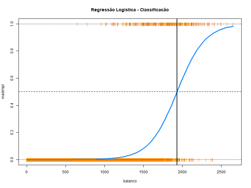
Curva S
# Mostrar a curva S com o resultado da regressão logística # Salvar o gráfico em um arquivo .png png ( "regressao_logistica.png" , width = 800 , height = 600 ) inadimpl <- as.numeric ( conj_treino $ inadimplente ) - 1 plot ( inadimpl ~ balanco , data = conj_treino , col = "darkorange" , pch = "|" , ylim = c ( 0 , 1 ) , main = "Regressão Logistica - Classificacão" ) abline ( h = 0 , lty = 3 ) abline ( h = 1 , lty = 3 ) abline ( h = 0.5 , lty = 2 ) curve ( predict ( mod1 , data.frame ( balanco = x ) , type = "response" ) , add = TRUE , lwd = 3 , col = "dodgerblue" ) abline ( v = - coef ( mod1 ) [ 1 ] / coef ( mod1 ) [ 2 ] , lwd = 2 ) dev.off ( )
2a Regressão logística: todas as variáveis
mod2 <- glm ( inadimplente ~ balanco + receita + estudante ,data= conj_treino ,family= binomial ) summary ( mod2 )
#>
#> Call:
#> glm(formula = inadimplente ~ balanco + receita + estudante, family = binomial,
#>     data = conj_treino)
#>
#> Coefficients:
#>               Estimate Std. Error z value Pr(>|z|)
#> (Intercept) -1.100e+01  5.277e-01 -20.850   <2e-16 ***
#> balanco      5.810e-03  2.488e-04  23.356   <2e-16 ***
#> receita      2.751e-06  8.799e-06   0.313   0.7546
#> estudante   -5.942e-01  2.516e-01  -2.362   0.0182 *
#> ---
#> Signif. codes:  0 '***' 0.001 '**' 0.01 '*' 0.05 '.' 0.1 ' ' 1
#>
#> (Dispersion parameter for binomial family taken to be 1)
#>
#>     Null deviance: 2623.8  on 8998  degrees of freedom
#> Residual deviance: 1396.8  on 8995  degrees of freedom
#> AIC: 1404.8
#>
#> Number of Fisher Scoring iterations: 8
#>   (Intercept)       balanco       receita     estudante
#> -1.100205e+01  5.810150e-03  2.750839e-06 -5.942048e-01
#>                  Estimate   Std. Error     z value      Pr(>|z|)
#> (Intercept) -1.100205e+01 5.276811e-01 -20.8498149  1.530134e-96
#> balanco      5.810150e-03 2.487659e-04  23.3558946 1.200621e-120
#> receita      2.750839e-06 8.798705e-06   0.3126414  7.545531e-01
#> estudante   -5.942048e-01 2.515801e-01  -2.3618911  1.818198e-02
É possível se ver que receita não é significativa
3a Regressão Logística (sem receita)
mod3 <- glm ( inadimplente ~ balanco + estudante ,data= conj_treino ,family= binomial ) summary ( mod3 )
#>
#> Call:
#> glm(formula = inadimplente ~ balanco + estudante, family = binomial,
#>     data = conj_treino)
#>
#> Coefficients:
#>               Estimate Std. Error z value Pr(>|z|)
#> (Intercept) -1.089e+01  3.974e-01 -27.416  < 2e-16 ***
#> balanco      5.812e-03  2.487e-04  23.368  < 2e-16 ***
#> estudante   -6.561e-01  1.550e-01  -4.234  2.3e-05 ***
#> ---
#> Signif. codes:  0 '***' 0.001 '**' 0.01 '*' 0.05 '.' 0.1 ' ' 1
#>
#> (Dispersion parameter for binomial family taken to be 1)
#>
#>     Null deviance: 2623.8  on 8998  degrees of freedom
#> Residual deviance: 1396.9  on 8996  degrees of freedom
#> AIC: 1402.9
#>
#> Number of Fisher Scoring iterations: 8
#>   (Intercept)       balanco     estudante
#> -10.894208021   0.005811976  -0.656054023
#>                  Estimate   Std. Error   z value      Pr(>|z|)
#> (Intercept) -10.894208021 0.3973729389 -27.41558 1.788553e-165
#> balanco       0.005811976 0.0002487146  23.36806 9.031818e-121
#> estudante    -0.656054023 0.1549533866  -4.23388  2.296937e-05
Comparando os modelos
anova ( mod2 ,mod3 ,test= 'LR' )
#> Analysis of Deviance Table
#>
#> Model 1: inadimplente ~ balanco + receita + estudante
#> Model 2: inadimplente ~ balanco + estudante
#>   Resid. Df Resid. Dev Df  Deviance Pr(>Chi)
#> 1      8995     1396.8
#> 2      8996     1396.9 -1 -0.097739   0.7546
StepAIC
Ao invé de usarmos a estatística de Wald para selecionar as variáveis significativas, podemos usar o AIC (equivalente ao Cp ) como usamos na regressão múltipla para selecionar as variáveis explicativas.
A função stepAIC tem um parametro k que define se vamos usar o AIC ou o BIC para fazer a seleção. Quando k=2 temos o AIC e quando k=log(n) temos o BIC.
#>
#> Call:
#> glm(formula = inadimplente ~ balanco + estudante, family = binomial,
#>     data = conj_treino)
#>
#> Coefficients:
#>               Estimate Std. Error z value Pr(>|z|)
#> (Intercept) -1.089e+01  3.974e-01 -27.416  < 2e-16 ***
#> balanco      5.812e-03  2.487e-04  23.368  < 2e-16 ***
#> estudante   -6.561e-01  1.550e-01  -4.234  2.3e-05 ***
#> ---
#> Signif. codes:  0 '***' 0.001 '**' 0.01 '*' 0.05 '.' 0.1 ' ' 1
#>
#> (Dispersion parameter for binomial family taken to be 1)
#>
#>     Null deviance: 2623.8  on 8998  degrees of freedom
#> Residual deviance: 1396.9  on 8996  degrees of freedom
#> AIC: 1402.9
#>
#> Number of Fisher Scoring iterations: 8
#>
#> Call:
#> glm(formula = inadimplente ~ balanco + estudante, family = binomial,
#>     data = conj_treino)
#>
#> Coefficients:
#>               Estimate Std. Error z value Pr(>|z|)
#> (Intercept) -1.089e+01  3.974e-01 -27.416  < 2e-16 ***
#> balanco      5.812e-03  2.487e-04  23.368  < 2e-16 ***
#> estudante   -6.561e-01  1.550e-01  -4.234  2.3e-05 ***
#> ---
#> Signif. codes:  0 '***' 0.001 '**' 0.01 '*' 0.05 '.' 0.1 ' ' 1
#>
#> (Dispersion parameter for binomial family taken to be 1)
#>
#>     Null deviance: 2623.8  on 8998  degrees of freedom
#> Residual deviance: 1396.9  on 8996  degrees of freedom
#> AIC: 1402.9
#>
#> Number of Fisher Scoring iterations: 8
Avaliando o modelo novamente
p_chapeu <- predict ( mod3 , newdata = conj_teste , type = "response" ) y_chapeu <- ifelse ( p_chapeu > 0.5 , "Sim" , "Nao" ) %>% factor ( levels = levels ( conj_teste $ inadimplente ) ) confusionMatrix ( y_chapeu , conj_teste $ inadimplente , positive= "Sim" )
#> Confusion Matrix and Statistics
#>
#>           Reference
#> Prediction Nao Sim
#>        Nao 960  24
#>        Sim   7  10
#>
#>                Accuracy : 0.969
#>                  95% CI : (0.9563, 0.9789)
#>     No Information Rate : 0.966
#>     P-Value [Acc > NIR] : 0.339451
#>
#>                   Kappa : 0.3781
#>
#>  Mcnemar's Test P-Value : 0.004057
#>
#>             Sensitivity : 0.29412
#>             Specificity : 0.99276
#>          Pos Pred Value : 0.58824
#>          Neg Pred Value : 0.97561
#>              Prevalence : 0.03397
#>          Detection Rate : 0.00999
#>    Detection Prevalence : 0.01698
#>       Balanced Accuracy : 0.64344
#>
#>        'Positive' Class : Sim
#>
Mudando a probabilidade (limite) para aumentar a sensibilidade
p_chapeu <- predict ( mod3 , newdata = conj_teste , type = "response" ) y_chapeu <- ifelse ( p_chapeu > 0.1 , "Sim" , "Nao" ) %>% factor ( levels = levels ( conj_teste $ inadimplente ) )
confusionMatrix ( y_chapeu , conj_teste $ inadimplente , positive= "Sim" )
#> Confusion Matrix and Statistics
#>
#>           Reference
#> Prediction Nao Sim
#>        Nao 912  11
#>        Sim  55  23
#>
#>                Accuracy : 0.9341
#>                  95% CI : (0.9169, 0.9486)
#>     No Information Rate : 0.966
#>     P-Value [Acc > NIR] : 1
#>
#>                   Kappa : 0.3815
#>
#>  Mcnemar's Test P-Value : 1.204e-07
#>
#>             Sensitivity : 0.67647
#>             Specificity : 0.94312
#>          Pos Pred Value : 0.29487
#>          Neg Pred Value : 0.98808
#>              Prevalence : 0.03397
#>          Detection Rate : 0.02298
#>    Detection Prevalence : 0.07792
#>       Balanced Accuracy : 0.80980
#>
#>        'Positive' Class : Sim
#>
Melhor limite
m_limite <- coords ( roc_log2 , "best" , ret = "threshold" ) $ threshold m_limite p_chapeu <- predict ( mod3 , newdata = conj_teste , type = "response" ) y_chapeu <- ifelse ( p_chapeu > m_limite , "Sim" , "Nao" ) %>% factor ( levels = levels ( conj_teste $ inadimplente ) )
confusionMatrix ( y_chapeu , conj_teste $ inadimplente , positive= "Sim" )
#> Confusion Matrix and Statistics
#>
#>           Reference
#> Prediction Nao Sim
#>        Nao 857   5
#>        Sim 110  29
#>
#>                Accuracy : 0.8851
#>                  95% CI : (0.8637, 0.9042)
#>     No Information Rate : 0.966
#>     P-Value [Acc > NIR] : 1
#>
#>                   Kappa : 0.2969
#>
#>  Mcnemar's Test P-Value : <2e-16
#>
#>             Sensitivity : 0.85294
#>             Specificity : 0.88625
#>          Pos Pred Value : 0.20863
#>          Neg Pred Value : 0.99420
#>              Prevalence : 0.03397
#>          Detection Rate : 0.02897
#>    Detection Prevalence : 0.13886
#>       Balanced Accuracy : 0.86959
#>
#>        'Positive' Class : Sim
#>
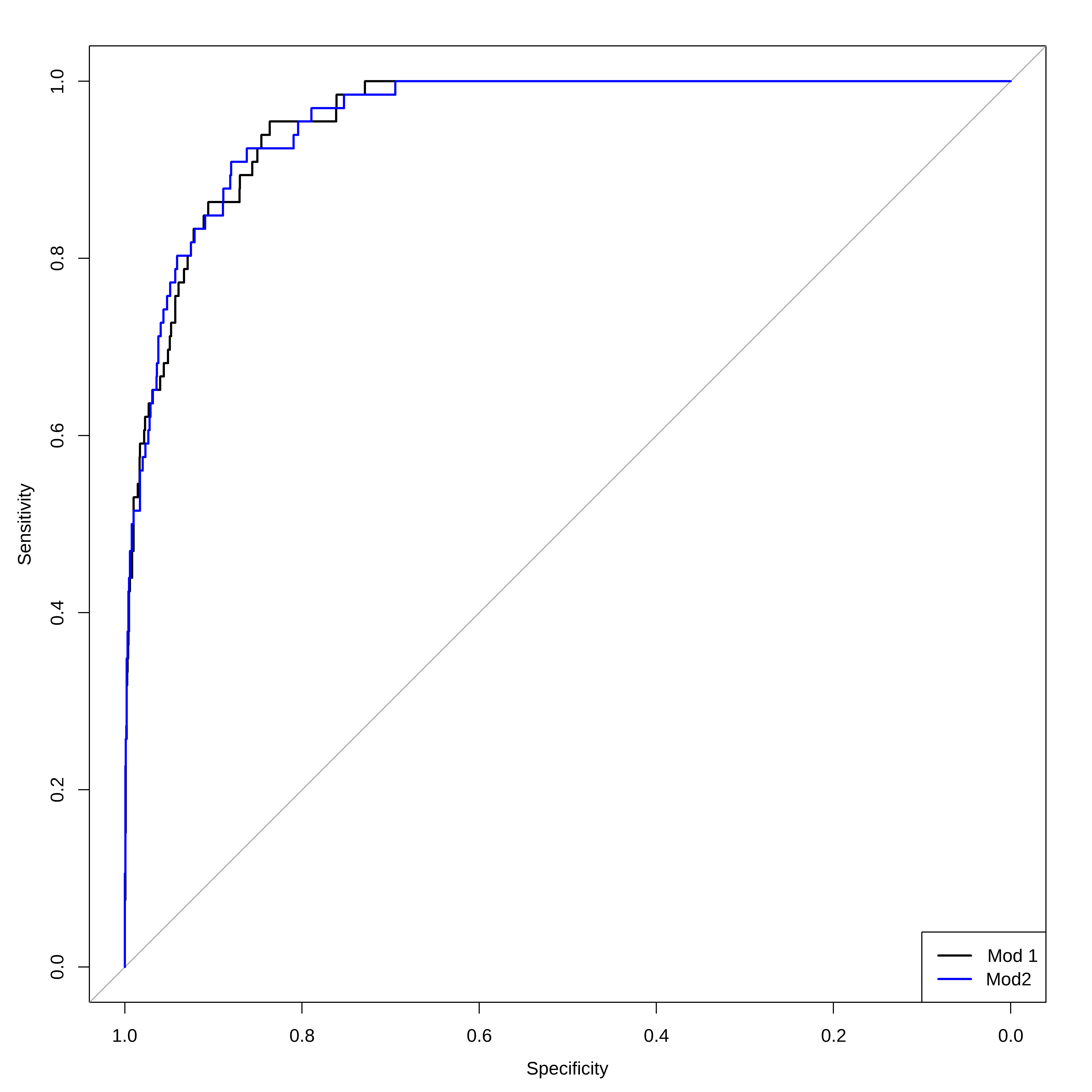
Duas ROCs juntas
# Visualização com ggroc ggroc ( list ( reglog1= roc_log , reglog2= roc_log2 ) ) + ggplot2 :: labs ( title = "ROC - Regressão Logística" , x = "1 - Especificidade" , y = "Sensibilidade" ) +
ggplot2 :: theme_minimal ( )
Reprodutibilidade
#> R version 4.5.1 (2025-06-13 ucrt)
#> Platform: x86_64-w64-mingw32/x64
#> Running under: Windows 11 x64 (build 26200)
#>
#> Matrix products: default
#>   LAPACK version 3.12.1
#>
#> locale:
#> [1] LC_COLLATE=Portuguese_Brazil.utf8  LC_CTYPE=Portuguese_Brazil.utf8
#> [3] LC_MONETARY=Portuguese_Brazil.utf8 LC_NUMERIC=C
#> [5] LC_TIME=Portuguese_Brazil.utf8
#>
#> time zone: America/Sao_Paulo
#> tzcode source: internal
#>
#> attached base packages:
#> [1] stats     graphics  grDevices utils     datasets  methods   base
#>
#> other attached packages:
#>  [1] MASS_7.3-65     ISLR_1.4        pROC_1.19.0.1   patchwork_1.3.1
#>  [5] caret_7.0-1     lattice_0.22-7  lubridate_1.9.4 forcats_1.0.0
#>  [9] stringr_1.5.1   dplyr_1.1.4     purrr_1.1.0     readr_2.1.5
#> [13] tidyr_1.3.1     tibble_3.3.0    ggplot2_3.5.2   tidyverse_2.0.0
#>
#> loaded via a namespace (and not attached):
#>  [1] gtable_0.3.6         xfun_0.52            htmlwidgets_1.6.4
#>  [4] recipes_1.3.1        tzdb_0.5.0           vctrs_0.6.5
#>  [7] tools_4.5.1          generics_0.1.4       stats4_4.5.1
#> [10] parallel_4.5.1       proxy_0.4-27         ModelMetrics_1.2.2.2
#> [13] pkgconfig_2.0.3      Matrix_1.7-3         data.table_1.17.8
#> [16] RColorBrewer_1.1-3   lifecycle_1.0.4      compiler_4.5.1
#> [19] farver_2.1.2         codetools_0.2-20     htmltools_0.5.8.1
#> [22] class_7.3-23         yaml_2.3.10          prodlim_2025.04.28
#> [25] pillar_1.11.0        gower_1.0.2          iterators_1.0.14
#> [28] rpart_4.1.24         foreach_1.5.2        nlme_3.1-168
#> [31] parallelly_1.45.1    lava_1.8.1           tidyselect_1.2.1
#> [34] digest_0.6.37        stringi_1.8.7        future_1.67.0
#> [37] reshape2_1.4.4       listenv_0.9.1        labeling_0.4.3
#> [40] splines_4.5.1        fastmap_1.2.0        grid_4.5.1
#> [43] cli_3.6.5            magrittr_2.0.3       dichromat_2.0-0.1
#> [46] survival_3.8-3       e1071_1.7-16         future.apply_1.20.0
#> [49] withr_3.0.2          scales_1.4.0         timechange_0.3.0
#> [52] rmarkdown_2.29       globals_0.18.0       nnet_7.3-20
#> [55] timeDate_4041.110    hms_1.1.3            evaluate_1.0.4
#> [58] knitr_1.50           hardhat_1.4.1        rlang_1.1.6
#> [61] Rcpp_1.1.0           glue_1.8.0           ipred_0.9-15
#> [64] rstudioapi_0.17.1    jsonlite_2.0.0       R6_2.6.1
#> [67] plyr_1.8.9