Carregando Bibliotecas
#>  default    student       balance           income
#>  No :9667   No :7056   Min.   :   0.0   Min.   :  772
#>  Yes: 333   Yes:2944   1st Qu.: 481.7   1st Qu.:21340
#>                        Median : 823.6   Median :34553
#>                        Mean   : 835.4   Mean   :33517
#>                        3rd Qu.:1166.3   3rd Qu.:43808
#>                        Max.   :2654.3   Max.   :73554
#> 'data.frame':    10000 obs. of  4 variables:
#>  $ default: Factor w/ 2 levels "No","Yes": 1 1 1 1 1 1 1 1 1 1 ...
#>  $ student: Factor w/ 2 levels "No","Yes": 1 2 1 1 1 2 1 2 1 1 ...
#>  $ balance: num  730 817 1074 529 786 ...
#>  $ income : num  44362 12106 31767 35704 38463 ...
#>   default student   balance    income
#> 1      No      No  729.5265 44361.625
#> 2      No     Yes  817.1804 12106.135
#> 3      No      No 1073.5492 31767.139
#> 4      No      No  529.2506 35704.494
#> 5      No      No  785.6559 38463.496
#> 6      No     Yes  919.5885  7491.559
Manipulando os dados
#>  default    student       balance           income
#>  No :9667   No :7056   Min.   :   0.0   Min.   :  772
#>  Yes: 333   Yes:2944   1st Qu.: 481.7   1st Qu.:21340
#>                        Median : 823.6   Median :34553
#>                        Mean   : 835.4   Mean   :33517
#>                        3rd Qu.:1166.3   3rd Qu.:43808
#>                        Max.   :2654.3   Max.   :73554
# renomeando colunas credito <- credito %>% rename ( inadimplente = default , estudante = student , balanco = balance ,
receita = income )
credito <- credito %>% mutate ( inadimplente = case_when ( inadimplente == "No" ~ "Nao" ,
inadimplente == "Yes" ~ "Sim"
) ) %>% mutate ( inadimplente = factor ( inadimplente ) )
credito <- credito %>% mutate ( estudante = case_when ( estudante == "No" ~ 0 ,
estudante == "Yes" ~ 1
) )
str ( credito )
#> tibble [10,000 × 4] (S3: tbl_df/tbl/data.frame)
#>  $ inadimplente: Factor w/ 2 levels "Nao","Sim": 1 1 1 1 1 1 1 1 1 1 ...
#>  $ estudante   : num [1:10000] 0 1 0 0 0 1 0 1 0 0 ...
#>  $ balanco     : num [1:10000] 730 817 1074 529 786 ...
#>  $ receita     : num [1:10000] 44362 12106 31767 35704 38463 ...
#>  inadimplente   estudante         balanco          receita
#>  Nao:9667     Min.   :0.0000   Min.   :   0.0   Min.   :  772
#>  Sim: 333     1st Qu.:0.0000   1st Qu.: 481.7   1st Qu.:21340
#>               Median :0.0000   Median : 823.6   Median :34553
#>               Mean   :0.2944   Mean   : 835.4   Mean   :33517
#>               3rd Qu.:1.0000   3rd Qu.:1166.3   3rd Qu.:43808
#>               Max.   :1.0000   Max.   :2654.3   Max.   :73554
Treino e Teste
set.seed ( 2025 ) y <- credito $ inadimplente indice_teste <- createDataPartition ( y , times = 1 , p = 0.1 , list = FALSE ) conj_treino <- credito [ - indice_teste ,] conj_teste <- credito [ indice_teste ,] summary ( conj_treino )
#>  inadimplente   estudante         balanco          receita
#>  Nao:8700     Min.   :0.0000   Min.   :   0.0   Min.   :  772
#>  Sim: 299     1st Qu.:0.0000   1st Qu.: 483.6   1st Qu.:21343
#>               Median :0.0000   Median : 821.3   Median :34576
#>               Mean   :0.2946   Mean   : 836.3   Mean   :33556
#>               3rd Qu.:1.0000   3rd Qu.:1167.1   3rd Qu.:43854
#>               Max.   :1.0000   Max.   :2654.3   Max.   :73554
#>  inadimplente   estudante         balanco          receita
#>  Nao:967      Min.   :0.0000   Min.   :   0.0   Min.   : 5386
#>  Sim: 34      1st Qu.:0.0000   1st Qu.: 453.6   1st Qu.:21319
#>               Median :0.0000   Median : 839.9   Median :34086
#>               Mean   :0.2927   Mean   : 827.4   Mean   :33170
#>               3rd Qu.:1.0000   3rd Qu.:1156.3   3rd Qu.:42856
#>               Max.   :1.0000   Max.   :2221.0   Max.   :70701
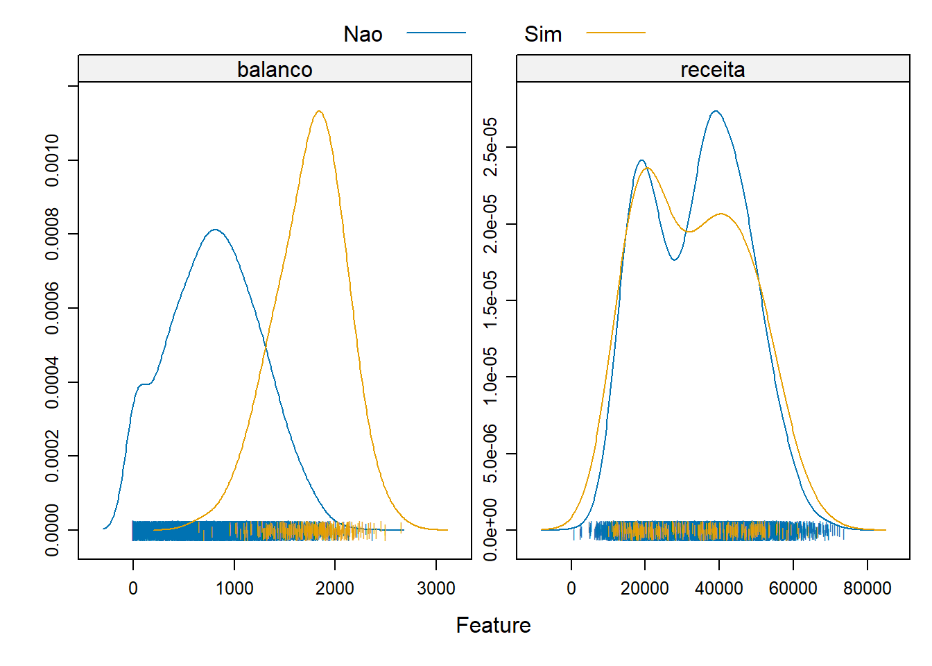
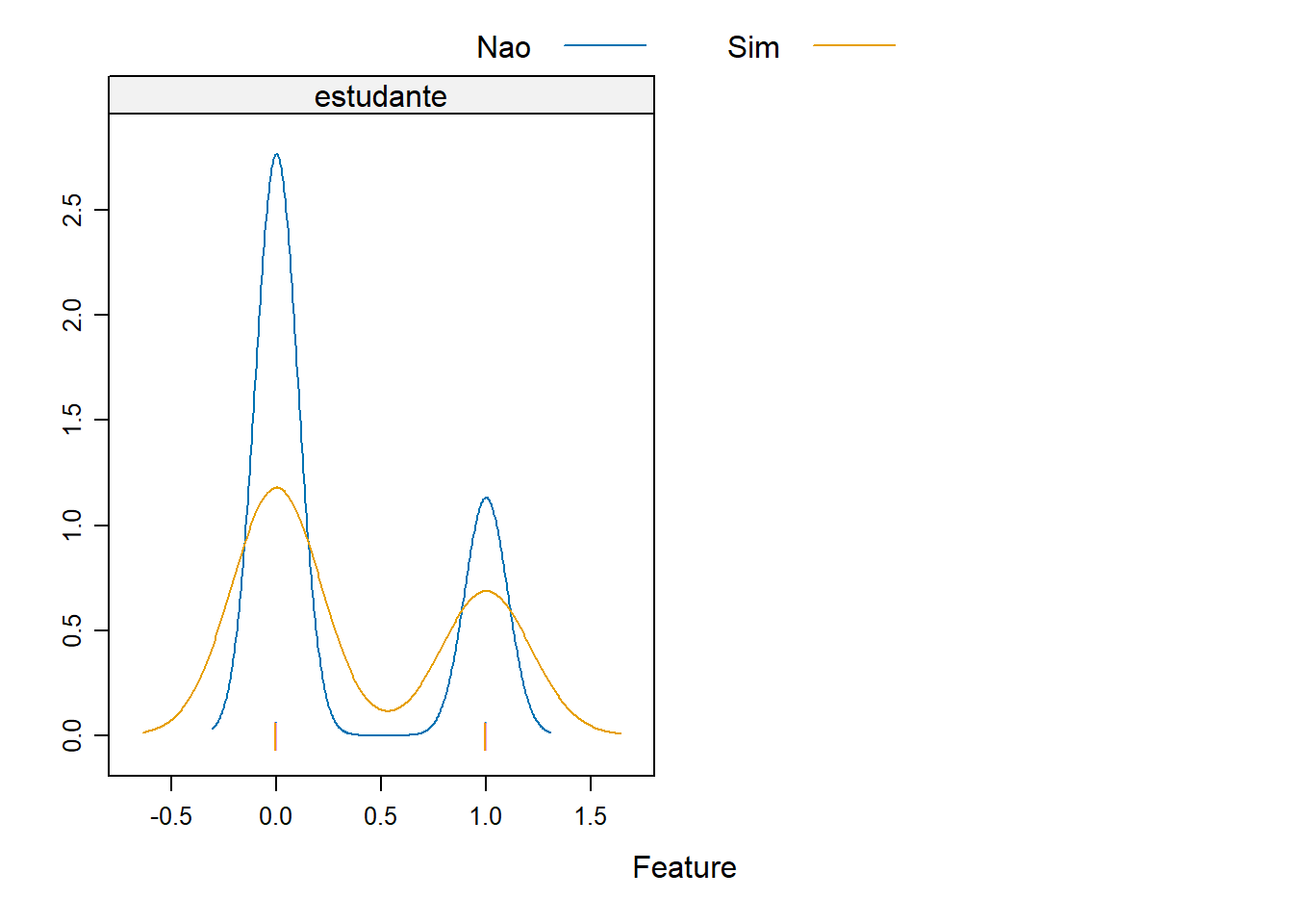
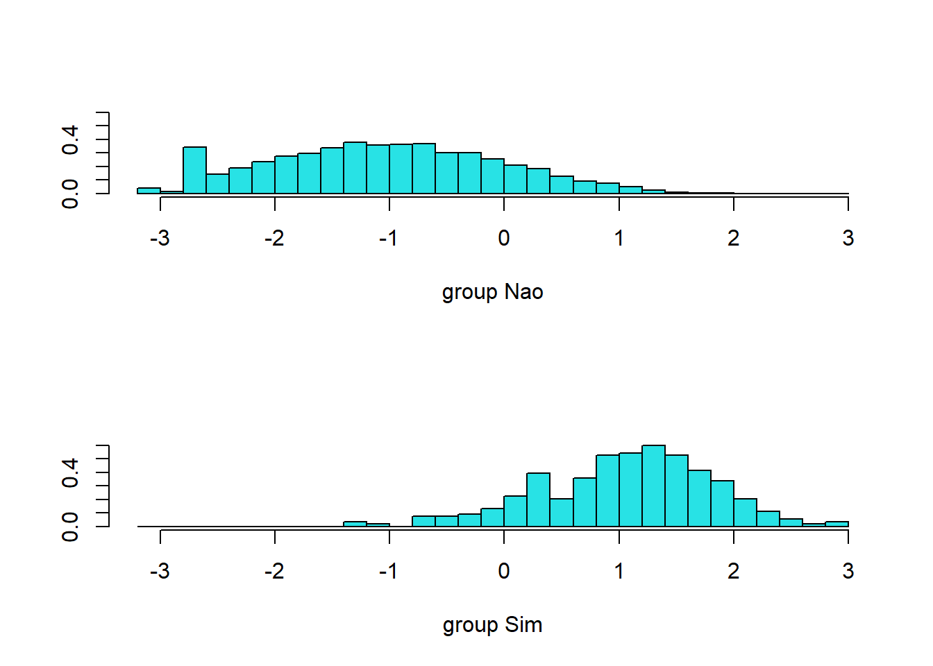
Graficos de Densidade
Vamos agora explorar os dados originais para termos algum visão do comportamento das variáveis explicativas e a variável dependente.
featurePlot ( x = conj_treino [ , c ( "balanco" , "receita" , "estudante" ) ] , y = conj_treino $ inadimplente ,
plot = "density" ,
scales = list ( x = list ( relation = "free" ) ,
y = list ( relation = "free" ) ) ,
adjust = 1.5 ,
pch = "|" ,
layout = c ( 2 , 1 ) ,
auto.key = list ( columns = 2 ) )
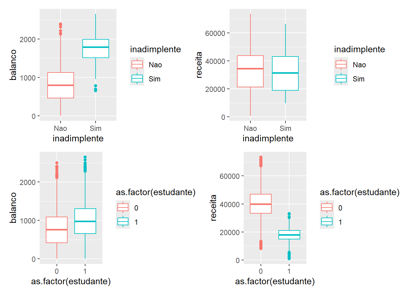
Avaliando o comportamento das variáveis em função do status (inadimplente / estudante)
p1 <- ggplot ( credito , aes ( x= inadimplente , y= balanco , color= inadimplente ) ) + geom_boxplot ( )
p2 <- ggplot ( credito , aes ( x= inadimplente , y= receita , color= inadimplente ) ) + geom_boxplot ( )
p3 <- ggplot ( credito , aes ( x= as.factor ( estudante ) , y= balanco , color= as.factor ( estudante ) ) ) + geom_boxplot ( )
p4 <- ggplot ( credito , aes ( x= as.factor ( estudante ) , y= receita , color= as.factor ( estudante ) ) ) + geom_boxplot ( )
( p1 + p2 ) / ( p3 + p4 )
Calcula Erro
# Este valor é igual a 1 - Accuracy da matriz de confusão calc_erro_class <- function ( real , previsto ) { mean ( real != previsto )
}
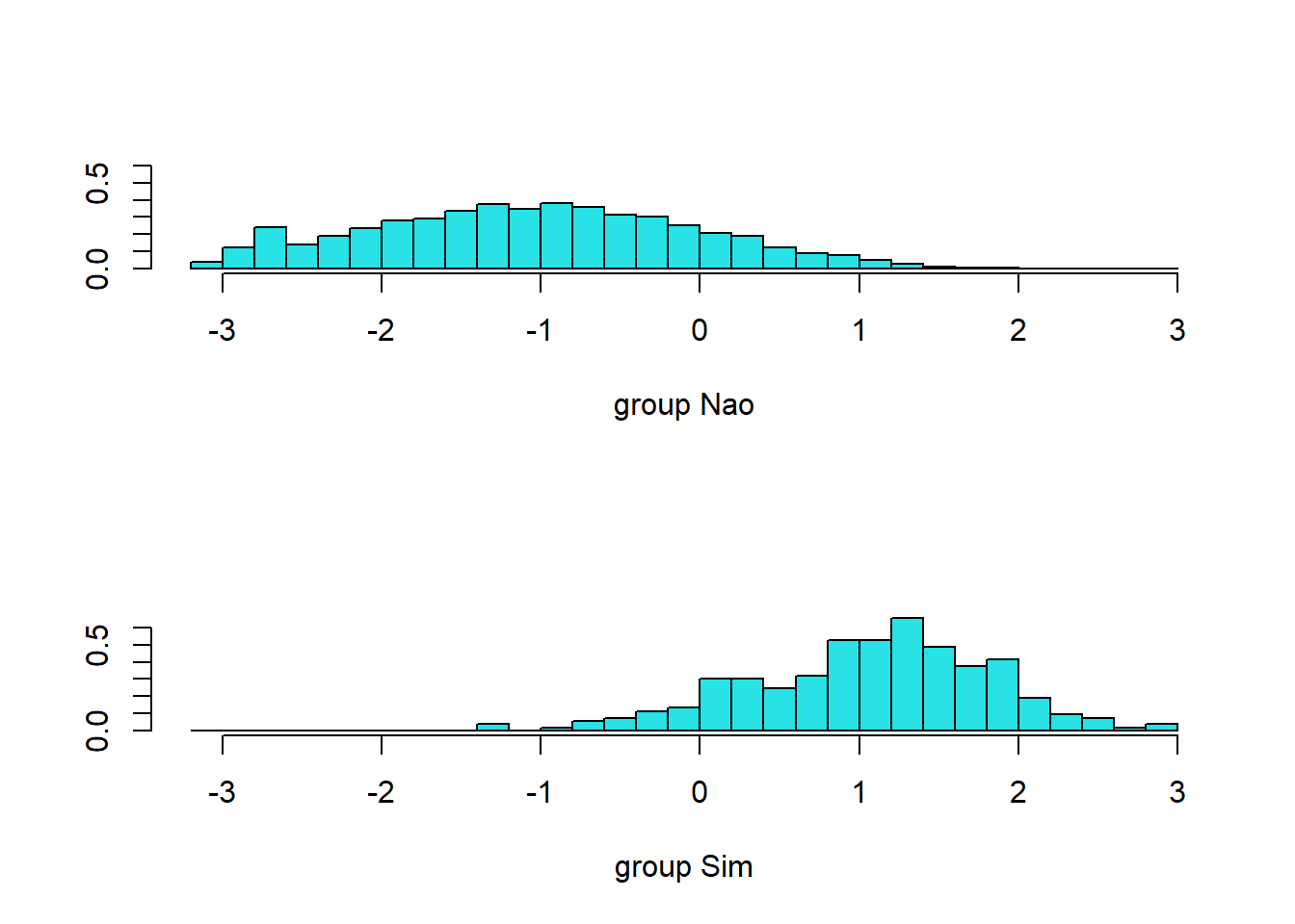
Treino e Teste Normalizado
set.seed ( 2025 ) y <- credito $ inadimplente indice_teste <- createDataPartition ( y , times = 1 , p = 0.1 , list = FALSE ) conj_treino <- credito [ - indice_teste ,] conj_teste <- credito [ indice_teste ,] # Normalizando os dados conj_treino <- conj_treino %>% mutate ( balanco = scale ( balanco ) , receita = scale ( receita ) ) conj_teste <- conj_teste %>% mutate ( balanco = scale ( balanco ) , receita = scale ( receita ) ) summary ( conj_treino )
#>  inadimplente   estudante              balanco.V1
#>  Nao:8700     Min.   :0.0000   Min.   :-1.7300270107000
#>  Sim: 299     1st Qu.:0.0000   1st Qu.:-0.7295373596360
#>               Median :0.0000   Median :-0.0310441386634
#>               Mean   :0.2946   Mean   : 0.0000000000000
#>               3rd Qu.:1.0000   3rd Qu.: 0.6843749315700
#>               Max.   :1.0000   Max.   : 3.7611705051700
#>           receita.V1
#>  Min.   :-2.45336351564e+00
#>  1st Qu.:-9.13961444854e-01
#>  Median : 7.63972196653e-02
#>  Mean   :-1.00000000000e-16
#>  3rd Qu.: 7.70708544207e-01
#>  Max.   : 2.99329553226e+00
#>  inadimplente   estudante               balanco.V1
#>  Nao:967      Min.   :0.0000   Min.   :-1.69939601081e+00
#>  Sim: 34      1st Qu.:0.0000   1st Qu.:-7.67712234966e-01
#>               Median :0.0000   Median : 2.55178067289e-02
#>               Mean   :0.2927   Mean   : 1.00000000000e-16
#>               3rd Qu.:1.0000   3rd Qu.: 6.75365461448e-01
#>               Max.   :1.0000   Max.   : 2.86197439052e+00
#>           receita.V1
#>  Min.   :-2.12068962027e+00
#>  1st Qu.:-9.04544180980e-01
#>  Median : 6.99730599216e-02
#>  Mean   :-2.00000000000e-16
#>  3rd Qu.: 7.39364666078e-01
#>  Max.   : 2.86470846852e+00
LDA
library ( MASS ) treina_lda <- lda ( inadimplente ~ balanco + estudante + receita , data = conj_treino ) treina_lda
#> Call:
#> lda(inadimplente ~ balanco + estudante + receita, data = conj_treino)
#>
#> Prior probabilities of groups:
#>        Nao        Sim
#> 0.96677409 0.03322591
#>
#> Group means:
#>         balanco estudante      receita
#> Nao -0.06531638 0.2911494  0.004454893
#> Sim  1.90051018 0.3946488 -0.129623970
#>
#> Coefficients of linear discriminants:
#>                   LD1
#> balanco    1.08468641
#> estudante -0.13706793
#> receita    0.04905863
#> [1] "class" "posterior" "x"
y_chapeu <- predict ( treina_lda , conj_teste ) $ class %>% factor ( levels = levels ( conj_teste $ inadimplente ) )
confusionMatrix ( data = y_chapeu , reference = conj_teste $ inadimplente , positive= "Sim" )
#> Confusion Matrix and Statistics
#>
#>           Reference
#> Prediction Nao Sim
#>        Nao 963  26
#>        Sim   4   8
#>
#>                Accuracy : 0.97
#>                  95% CI : (0.9575, 0.9797)
#>     No Information Rate : 0.966
#>     P-Value [Acc > NIR] : 0.276410
#>
#>                   Kappa : 0.3361
#>
#>  Mcnemar's Test P-Value : 0.000126
#>
#>             Sensitivity : 0.235294
#>             Specificity : 0.995863
#>          Pos Pred Value : 0.666667
#>          Neg Pred Value : 0.973711
#>              Prevalence : 0.033966
#>          Detection Rate : 0.007992
#>    Detection Prevalence : 0.011988
#>       Balanced Accuracy : 0.615579
#>
#>        'Positive' Class : Sim
#>
# Este valor é igual a 1 - Accuracy da matriz de confusão calc_erro_class ( conj_teste $ inadimplente , y_chapeu )
LDA - Ajustando probabilidade limite
p_chapeu <- predict ( treina_lda , conj_teste ) $ posterior head ( p_chapeu )
#>         Nao          Sim
#> 1 0.9880289 0.0119710647
#> 2 0.9990743 0.0009256652
#> 3 0.9959870 0.0040130108
#> 4 0.9914601 0.0085398543
#> 5 0.9867357 0.0132643344
#> 6 0.9980803 0.0019196683
y_chapeu <- ifelse ( p_chapeu [ , 2 ] > 0.11 , "Sim" , "Nao" ) %>% factor ( levels = levels ( conj_teste $ inadimplente ) )
confusionMatrix ( data = y_chapeu , reference = conj_teste $ inadimplente , positive= "Sim" )
#> Confusion Matrix and Statistics
#>
#>           Reference
#> Prediction Nao Sim
#>        Nao 912  11
#>        Sim  55  23
#>
#>                Accuracy : 0.9341
#>                  95% CI : (0.9169, 0.9486)
#>     No Information Rate : 0.966
#>     P-Value [Acc > NIR] : 1
#>
#>                   Kappa : 0.3815
#>
#>  Mcnemar's Test P-Value : 1.204e-07
#>
#>             Sensitivity : 0.67647
#>             Specificity : 0.94312
#>          Pos Pred Value : 0.29487
#>          Neg Pred Value : 0.98808
#>              Prevalence : 0.03397
#>          Detection Rate : 0.02298
#>    Detection Prevalence : 0.07792
#>       Balanced Accuracy : 0.80980
#>
#>        'Positive' Class : Sim
#>
# Este valor é igual a 1 - Accuracy da matriz de confusão calc_erro_class ( conj_teste $ inadimplente , y_chapeu )
Seleção de variáveis
No LDA, a seleção de variáveis pode ser feita com o RFE (Recursive Feature Elimination). O RFE é um método de seleção de variáveis que utiliza a validação cruzada para avaliar o desempenho do modelo com diferentes subconjuntos de variáveis. O RFE é implementado na função rfe() caret.
# Usar o RFE para selecionar as variáveis # Definir controle para RFE control <- rfeControl ( functions = ldaFuncs , method = "cv" , number = 10 ) # Aplicar o RFE set.seed ( 2025 ) result <- rfe ( conj_treino [ , 2 : 4 ] , conj_treino $ inadimplente , sizes = c ( 1 : 3 ) , rfeControl = control ) # Resultados print ( result )
#>
#> Recursive feature selection
#>
#> Outer resampling method: Cross-Validated (10 fold)
#>
#> Resampling performance over subset size:
#>
#>  Variables Accuracy  Kappa AccuracySD KappaSD Selected
#>          1   0.9726 0.3487   0.002776  0.1048
#>          2   0.9728 0.3564   0.002634  0.1045        *
#>          3   0.9724 0.3396   0.002910  0.1153
#>
#> The top 2 variables (out of 2):
#>    balanco, estudante
Outra Opção
Podemos usar os gráfico exploratórios iniciais e também o resultado da regressão logística como ponto de partida para a seleção de variáveis.
treina_lda2 <- lda ( inadimplente ~ balanco + estudante , data = conj_treino ) treina_lda2
#> Call:
#> lda(inadimplente ~ balanco + estudante, data = conj_treino)
#>
#> Prior probabilities of groups:
#>        Nao        Sim
#> 0.96677409 0.03322591
#>
#> Group means:
#>         balanco estudante
#> Nao -0.06531638 0.2911494
#> Sim  1.90051018 0.3946488
#>
#> Coefficients of linear discriminants:
#>                  LD1
#> balanco    1.0850633
#> estudante -0.2183485
y_chapeu <- predict ( treina_lda2 , conj_teste ) $ class %>% factor ( levels = levels ( conj_teste $ inadimplente ) )
confusionMatrix ( data = y_chapeu , reference = conj_teste $ inadimplente , positive= "Sim" )
#> Confusion Matrix and Statistics
#>
#>           Reference
#> Prediction Nao Sim
#>        Nao 963  26
#>        Sim   4   8
#>
#>                Accuracy : 0.97
#>                  95% CI : (0.9575, 0.9797)
#>     No Information Rate : 0.966
#>     P-Value [Acc > NIR] : 0.276410
#>
#>                   Kappa : 0.3361
#>
#>  Mcnemar's Test P-Value : 0.000126
#>
#>             Sensitivity : 0.235294
#>             Specificity : 0.995863
#>          Pos Pred Value : 0.666667
#>          Neg Pred Value : 0.973711
#>              Prevalence : 0.033966
#>          Detection Rate : 0.007992
#>    Detection Prevalence : 0.011988
#>       Balanced Accuracy : 0.615579
#>
#>        'Positive' Class : Sim
#>
# Este valor é igual a 1 - Accuracy da matriz de confusão calc_erro_class ( conj_teste $ inadimplente , y_chapeu )
Podemos observar que não houve mudança nos resultados ao retirar a variável receita.
QDA
treina_qda <- qda ( inadimplente ~ balanco + estudante + receita , data = conj_treino ) treina_qda
#> Call:
#> qda(inadimplente ~ balanco + estudante + receita, data = conj_treino)
#>
#> Prior probabilities of groups:
#>        Nao        Sim
#> 0.96677409 0.03322591
#>
#> Group means:
#>         balanco estudante      receita
#> Nao -0.06531638 0.2911494  0.004454893
#> Sim  1.90051018 0.3946488 -0.129623970
y_chapeu <- predict ( treina_qda , conj_teste ) $ class %>% factor ( levels = levels ( conj_teste $ inadimplente ) )
confusionMatrix ( data = y_chapeu , reference = conj_teste $ inadimplente , positive= "Sim" )
#> Confusion Matrix and Statistics
#>
#>           Reference
#> Prediction Nao Sim
#>        Nao 961  25
#>        Sim   6   9
#>
#>                Accuracy : 0.969
#>                  95% CI : (0.9563, 0.9789)
#>     No Information Rate : 0.966
#>     P-Value [Acc > NIR] : 0.339451
#>
#>                   Kappa : 0.3539
#>
#>  Mcnemar's Test P-Value : 0.001225
#>
#>             Sensitivity : 0.264706
#>             Specificity : 0.993795
#>          Pos Pred Value : 0.600000
#>          Neg Pred Value : 0.974645
#>              Prevalence : 0.033966
#>          Detection Rate : 0.008991
#>    Detection Prevalence : 0.014985
#>       Balanced Accuracy : 0.629251
#>
#>        'Positive' Class : Sim
#>
QDA - Ajustando probabilidade limite
p_chapeu <- predict ( treina_qda , conj_teste ) $ posterior head ( p_chapeu )
#>         Nao          Sim
#> 1 0.9938988 6.101236e-03
#> 2 0.9999611 3.894230e-05
#> 3 0.9989868 1.013214e-03
#> 4 0.9956284 4.371627e-03
#> 5 0.9911388 8.861230e-03
#> 6 0.9999216 7.840825e-05
y_chapeu <- ifelse ( p_chapeu [ , 2 ] > 0.11 , "Sim" , "Nao" ) %>% factor ( levels = levels ( conj_teste $ inadimplente ) )
confusionMatrix ( data = y_chapeu , reference = conj_teste $ inadimplente , positive= "Sim" )
#> Confusion Matrix and Statistics
#>
#>           Reference
#> Prediction Nao Sim
#>        Nao 905  11
#>        Sim  62  23
#>
#>                Accuracy : 0.9271
#>                  95% CI : (0.9092, 0.9424)
#>     No Information Rate : 0.966
#>     P-Value [Acc > NIR] : 1
#>
#>                   Kappa : 0.3553
#>
#>  Mcnemar's Test P-Value : 4.855e-09
#>
#>             Sensitivity : 0.67647
#>             Specificity : 0.93588
#>          Pos Pred Value : 0.27059
#>          Neg Pred Value : 0.98799
#>              Prevalence : 0.03397
#>          Detection Rate : 0.02298
#>    Detection Prevalence : 0.08492
#>       Balanced Accuracy : 0.80618
#>
#>        'Positive' Class : Sim
#>
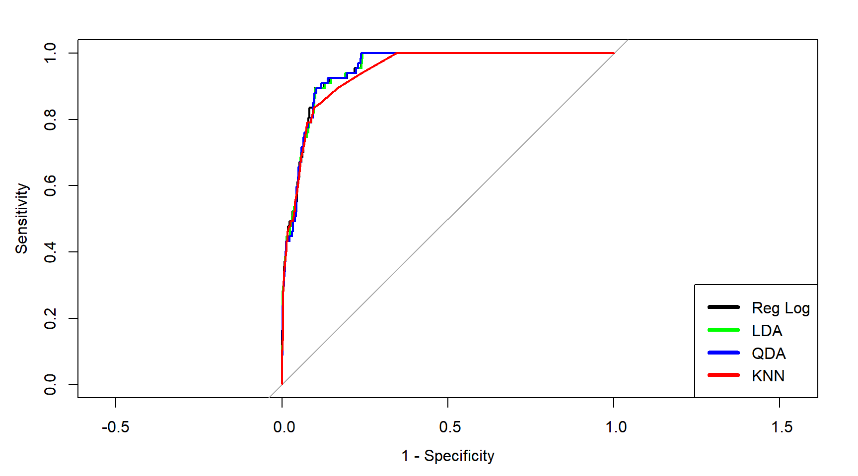
Curva ROC
# KNN set.seed ( 2025 ) ctrl <- trainControl ( method = "cv" ) treina_knn <- train ( inadimplente ~ balanco + estudante , method = "knn" , trControl= ctrl , preProcess= c ( "center" , "scale" ) , tuneGrid = data.frame ( k = seq ( 21 ,140 , by= 4 ) ) , data = conj_treino ) prev_knn <- predict ( treina_knn , conj_teste ,type = "prob" ) # Reg Log mod2 <- glm ( inadimplente ~ balanco + estudante ,data= conj_treino ,family= binomial ) p_chapeu_log <- predict ( mod2 , newdata = conj_teste , type = "response" ) # LDA e QDA p_chapeu_lda <- predict ( treina_lda , conj_teste ) $ posterior p_chapeu_qda <- predict ( treina_qda , conj_teste ) $ posterior roc_log <- roc ( conj_teste $ inadimplente ~ p_chapeu_log , print.auc= FALSE ) roc_lda <- roc ( conj_teste $ inadimplente ~ p_chapeu_lda [ ,2 ] , print.auc= FALSE ) roc_qda <- roc ( conj_teste $ inadimplente ~ p_chapeu_qda [ ,2 ] , print.auc= FALSE ) roc_knn1 <- roc ( conj_teste $ inadimplente ~ prev_knn [ ,2 ] , print.auc= FALSE ) # Visualização com ggroc ggroc ( list ( KNN= roc_knn1 , RegLog= roc_log , LDA= roc_lda , QDA= roc_qda ) ) + ggplot2 :: labs ( title = "ROC - KNN vs Reg Logística vs LDA vs QDA" , x = "1 - Especificidade" , y = "Sensibilidade" ) +
ggplot2 :: theme_minimal ( )
Reprodutibilidade
#> R version 4.5.1 (2025-06-13 ucrt)
#> Platform: x86_64-w64-mingw32/x64
#> Running under: Windows 11 x64 (build 26200)
#>
#> Matrix products: default
#>   LAPACK version 3.12.1
#>
#> locale:
#> [1] LC_COLLATE=Portuguese_Brazil.utf8  LC_CTYPE=Portuguese_Brazil.utf8
#> [3] LC_MONETARY=Portuguese_Brazil.utf8 LC_NUMERIC=C
#> [5] LC_TIME=Portuguese_Brazil.utf8
#>
#> time zone: America/Sao_Paulo
#> tzcode source: internal
#>
#> attached base packages:
#> [1] stats     graphics  grDevices utils     datasets  methods   base
#>
#> other attached packages:
#>  [1] MASS_7.3-65     ISLR_1.4        pROC_1.19.0.1   patchwork_1.3.1
#>  [5] caret_7.0-1     lattice_0.22-7  lubridate_1.9.4 forcats_1.0.0
#>  [9] stringr_1.5.1   dplyr_1.1.4     purrr_1.1.0     readr_2.1.5
#> [13] tidyr_1.3.1     tibble_3.3.0    ggplot2_3.5.2   tidyverse_2.0.0
#>
#> loaded via a namespace (and not attached):
#>  [1] gtable_0.3.6         xfun_0.52            htmlwidgets_1.6.4
#>  [4] recipes_1.3.1        tzdb_0.5.0           vctrs_0.6.5
#>  [7] tools_4.5.1          generics_0.1.4       stats4_4.5.1
#> [10] parallel_4.5.1       proxy_0.4-27         ModelMetrics_1.2.2.2
#> [13] pkgconfig_2.0.3      Matrix_1.7-3         data.table_1.17.8
#> [16] RColorBrewer_1.1-3   lifecycle_1.0.4      compiler_4.5.1
#> [19] farver_2.1.2         codetools_0.2-20     htmltools_0.5.8.1
#> [22] class_7.3-23         yaml_2.3.10          prodlim_2025.04.28
#> [25] pillar_1.11.0        gower_1.0.2          iterators_1.0.14
#> [28] rpart_4.1.24         foreach_1.5.2        nlme_3.1-168
#> [31] parallelly_1.45.1    lava_1.8.1           tidyselect_1.2.1
#> [34] digest_0.6.37        stringi_1.8.7        future_1.67.0
#> [37] reshape2_1.4.4       listenv_0.9.1        labeling_0.4.3
#> [40] splines_4.5.1        fastmap_1.2.0        grid_4.5.1
#> [43] cli_3.6.5            magrittr_2.0.3       dichromat_2.0-0.1
#> [46] survival_3.8-3       e1071_1.7-16         future.apply_1.20.0
#> [49] withr_3.0.2          scales_1.4.0         timechange_0.3.0
#> [52] rmarkdown_2.29       globals_0.18.0       nnet_7.3-20
#> [55] timeDate_4041.110    hms_1.1.3            evaluate_1.0.4
#> [58] knitr_1.50           hardhat_1.4.1        rlang_1.1.6
#> [61] Rcpp_1.1.0           glue_1.8.0           ipred_0.9-15
#> [64] rstudioapi_0.17.1    jsonlite_2.0.0       R6_2.6.1
#> [67] plyr_1.8.9